Image loading is done in a few mouse clicks (click the disk icon and select the image name from a list).
WinSCANOPY then displays the image on screen. |
| 2. Specify the region to analyse |
|
To analyse an image, you
must indicate which region is the hemisphere. This can be done by three methods:
a) The easiest method is
when you own a camera and lens calibrated and sold by Regent Instruments.
In this situation WinSCANOPYreads from our calibration file the necessary parameters to identify the
region to analyse, so the only thing you have to do to start the analysis
is to click the image. This file indicates to WinSCANOPYwhere is the centre of
the hemisphere, what is the radius that produces a 180 degrees field of
view and how to compensate for lens distortions. These parameters can be
overridden to reduce the field of view at the zenith or horizon for
example.
b) You can specify the
region to analyse interactively (Regular or Pro)
. You can move and resize the hemisphere
using mouse and keyboard keys commands. |
 |
|
| |
 |
|
c) You can specify the region
to analyse with numerical parameters (the centre position and radius size
in pixels). You can determine these experimentally. Although some freeware
manufacturers claim this step is "easy", you will have to invest
material resources and significant time to do this precisely (the final cost
often being larger than buying a complete calibrated system ready to use).
|
When you release the
mouse button after the hemisphere creation,WinSCANOPYautomatically displays
the sample identification window that allows you to set the information
specific to the image being analysed. You can customize this window's
information (choose which information is shown). Some of this information is used for the analysis, latitude and
longitude are used to calculate solar paths for example, while the rest is
simply reproduced in the data files along with the measurements. When you
click OK in this identification window, the analysis begins and is
displayed after completion.
The hemisphere’s diameter
and position in the image are also saved in the measurements data file so
these parameters can be verified after the analysis. The analysis data and
settings are also saved with the image (in the same tiff file) and can be
retrieved later by
WinSCANOPY to recreate the analysis. |
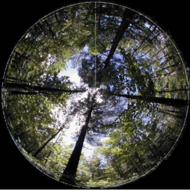
When the analysis is
complete, it is visible in the main window. The sky grid, divided in the number
of azimuthal and zenithal divisions that you choose, is displayed in
yellow. Messages to the operator and partial analysis data are displayed to
the left of the image. Detailes data are saved inWinSCANOPY's data files. |
Additional information
about a sky region can be displayed by clicking it in the image.
Suntracks, each
containing the sun’s position in the image for different hours of a
particular day, are displayed with rainbow-style colors (the color is
related to the intensity of the radiation level above the canopy). The date
is displayed close to it.
When you click a
suntrack, information about its closest point to the clicked position is
displayed. This includes the date, hour and instantaneous radiation value
for that moment. Its data are also displayed in the graphic above the image
and summarized to the left of the image.
Menus in the upper-right
corner of the graphic (all versions except Mini) allow you to select the
type of data and the relevant options you wish to be displayed. The available data are: |
| |
1) Radiation level per hour of the day for the active suntrack |
|
| |
 |
|
| |
2) Radiation level per day |
|
| |
 |
|
| |
3)Gap fractions in function of zenith or azimuthal direction |
|
| |
 |
|
| |
4) Leaf angle distribution |
|
| |
 |
|
| |
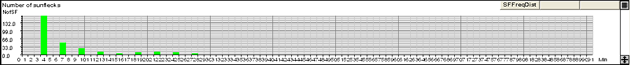
5) Sunfleck frequency distribution (number in function of duration in minutes) |
|
| |
 |
|
| |
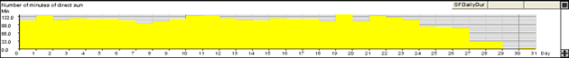
6) Sunfleck duration (total in minutes) per day of the growing season |
|
| |
 |
|
| |
7) Gaps size cumulative distribution |
|
| |
 |
|
| |
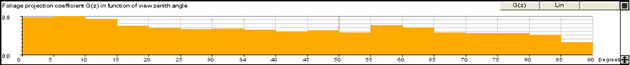
8) Leaf projection coefficient in function of zenith angle |
|
| |
 |
|
| |
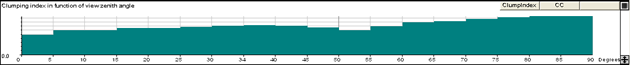
9) Clumping index in function of zenith angle |
|
| |
 |
|
At the end of the analysis,
data are automatically saved by WinSCANOPY in standard ASCII text
format that is well adapted to manipulation into spreadsheet programs like
Microsoft Excel. You have entire control on what is saved in data files (Regular, Pro).
You can choose to save or not:
- The settings used to analyse the image, information about the camera, lens and the analyses hemisphere position and size.
- The measurement data (LAI, Openness, Radiations...).
Data produced by WinSCANOPY fall into these categories (the list below is incomplete):
- Global data. These are measurements that have a single value for the entire image. Some examples of global data are
the site factors, openness, daily radiation for the growing season, leaf area index and NDVI data (Pro NDVI version only).
WinSCANOPY's analysis settings are also saved in the global data line along with the image information.
- Gap fractions per sky region, per elevation ring and per direction. Openness per elevation ring.
- Radiation per day. This include six data types: direct and indirect (diffuse), above and below canopy and total
radiation. Radiation is clearly presented by day and month (10 June 2000) and not by Julian or
decimal days (like day 322).
- Leaf angle density and cumulative leaf angle density.
- A table of the percentage of time that direct radiation is received at the photo location; per hour for each month.
- Sunfleck distribution and duration.
- Clumping index in function of zenith angle and per sky region.
- Leaf projection coefficient in function of zenith angle.
- Measured and theoretical gaps size distribution.
|
|